Seismic Modeling Analysis

Workflow summary: compute elastic attributes from the model, deriveangle-dependent reflectivity (Aki‑Richards / Zoeppritz), convolve with a Ricker wavelet, and produce time &depth seismograms. Use the domain selector and interactive viewers to inspect, compare, and export results.

AVO Analysis Characteristics

Quick tips: start with the full-stack to identify majorstructural features, then compare individual angle stacks to find zones where amplitude changes with offset.Use the domain selector to switch between depth-aligned rock-physics comparisons and time-domain TWT views forprocessing-style checks. Export angle stacks or attribute extracts for quantitative testing andmachine-learning experiments.

Methodology

The workflow computes reflectivity from elastic inputs,applies a Ricker wavelet, and produces analysis-ready synthetic volumes in both time and depth forinterpretation, attribute extraction, and method validation.

Amplitude Variation with Offset (AVO) modeling computesangle-dependent reflectivity at multiple incident angles (0°, 15°, 22.5°, and 30°) using the Zoeppritz equations. The approach exploits amplitude variations to infer lithology and fluid properties, withthe full-stack seismogram generated by combining all angle gathers into a composite trace.

Mathematical Framework

This section provides comprehensive technical specifications and implementation details for the AVO seismicmodeling workflow, including parameter configurations, computational methods, and practical guidance forreproducing and extending the analysis.

The mathematical foundation underlying AVO analysis quantifies how elastic properties influence seismicreflections at different angles, enabling the extraction of diagnostic attributes for reservoircharacterization.

Based on the Aki-Richards linearization of Zoeppritz equations for P-wave reflectioncoefficients:

The table below summarizes the practical strengths and known limitations of the Aki‑Richards / AVO approach as applied to the Stanford VI‑E synthetic dataset. Use this comparison to guide interpretation priorities and to understand where supplemental data or additional modeling may be required.

Seismic Data Products

A complete collection of multi‑angle synthetic seismic volumes in both time and depth domains, built foradvanced AVO interpretation and reservoir characterization workflows.

The Stanford VI‑E release provides physics‑based synthetic seismic products generated with rigorous AVO forwardmodeling. Available items include a full‑stack volume plus four angle stacks (0°, 15°, 22.5°, 30°),supplied in both two‑way travel time (TWT) and depth coordinates. These multi‑angle volumes preserveamplitude‑versus‑offset behavior required for fluid detection, lithology discrimination, attribute extraction, andquantitative interpretation. Each product includes technical metadata and interpretive notes to support reproducibleanalysis and method testing.

Full-Stack AVO Seismogram — the structural baseline

The full‑stack seismogram is a quality‑weighted integration of all angle contributions (0–30°) that producesthe familiar post‑stack image used for structural interpretation.

The full‑stack emphasizes strong impedance contrasts at major lithologic boundaries while suppressingangle‑dependent variability, making it an ideal first look at reservoir geometry. Inline, crossline andtime/depth slices expose anticlinal structure, layer continuity and internal heterogeneity. Use thefull‑stack as the reference baseline when comparing individual angle stacks or extracting AVO attributes.

Figure 4. Full-Stack AVO Seismogram - Integrated view combining all angle stacks (inline, crossline, and time slices)

Individual Angle Stacks

Four angle-specific seismic volumes (0°, 15°, 22.5°, 30°) that isolate how reflection amplitudes change withoffset, enabling focused AVO analysis and improved sensitivity to fluids and lithology.

Each angle stack is computed from the model using a linearized Zoeppritz formulation (Aki‑Richards) andemphasizes different physical responses. Near‑offset stacks (0–15°) are dominated by acoustic impedancecontrasts and provide the best structural image; mid‑to‑far offsets (22.5–30°) increase sensitivity toPoisson’s‑ratio and fluid effects. Comparing stacks across angles enables extraction of AVO attributes(intercept, gradient) for quantitative interpretation. Both time‑domain (TWT) and depth representations areavailable to support velocity‑aware analysis and direct comparison with rock‑physics attributes.

Figure 5. Angle Stack at 0° (Near Offset) - Normal incidence reflections

Figure 6. Angle Stack at 15° - Intermediate offset showing AVO effects

Figure 7. Angle Stack at 22.5° - Enhanced fluid sensitivity

Figure 8. Angle Stack at 30° (Far Offset) - Maximum AVO response

Implementation & Usage

This section provides comprehensive technical specifications and implementation details for the AVO seismicmodeling workflow, including parameter configurations, computational methods, and practical guidance forreproducing and extending the analysis.

Technical Implementation Details

This AVO analysis is based on a comprehensive seismic modeling configuration, starting with a detailed Grid Configuration. The model volume is defined by a 150x200x200 grid, which is finely sampled at 1 meter in depth (dz = 1 m) and 1 millisecond in time (dt = 1 ms). This dual-sampling provides high resolution for both the geological model and the resulting seismic data.

Key Seismic Parameters are used to generate the response. A standard 25 Hz Ricker wavelet serves as the source signal. The AVO response is modeled across a set of four discrete incidence angles: 0°, 15°, 22.5°, and 30°, enabling a robust analysis of angle-dependent reflectivity.

The core Methodology relies on the Aki-Richards linearization of the Zoeppritz equations, a standard and efficient industry approach for calculating reflectivity. The resulting angle gathers are then combined using full-stack integration to create the final volumes.

The Processing Workflow is designed for flexibility, featuring a bidirectional Depth-Time-Depth domain conversion. This allows the pipeline to generate dual seismogram outputs in both time and depth. Notably, the entire modeling process is highly efficient, completing in approximately 15 seconds.

Running the Code

To generate the AVO seismic volumes, run the primary modeling pipeline using the command python -m src --run-tool seismograms, which creates outputs in both the time and depth domains. For a complete workflow that also includes generating the corresponding visualizations, execute python -m src --run-tool analysis_seismograms. As a subsequent step, you can specifically analyze the correlation between the resulting seismic data and the geological facies by running python -m src --run-tool analyze_facies_correlation.

Generate AVO seismic volumes in both time and depth domains:

# Run AVO modeling pipeline (generates both domains)
python -m src --run-tool seismograms

# Complete seismic analysis with visualizations (both domains)
python -m src --run-tool analysis_seismograms

# Analyze facies-seismic correlation
python -m src --run-tool analyze_facies_correlation

AVO (Amplitude Versus Offset) attributes measure how seismic reflection amplitudes change with incidence angle. Intercept (A) captures the zero-offset reflection strength related to acoustic impedance contrast, while Gradient (B) describes the angular dependence often sensitive to elastic contrasts such as Poisson's ratio and fluid effects. Together, these attributes help discriminate lithology and fluids by separating impedance-driven amplitude from angle-dependent elastic responses.

Poisson's ratio and the Vp/Vs ratio are complementary elastic diagnostics: Poisson's ratio is sensitive to the relative compressibility of the rock matrix and pore fluids, while Vp/Vs highlights lithology and saturation contrasts. Together they improve discrimination between gas, oil, and brine-bearing rocks and help reduce ambiguities present when using single attributes alone.

With the physical interpretation and diagnostic applications of these rock physics attributes established, we now turn to the technical implementation details. Understanding the computation methods, mathematical formulations, and algorithmic workflows is essential for reproducibility, quality assurance, and proper interpretation of the attribute volumes derived from the fundamental elastic properties.

Rock Physics Attribute Volumes

Visualizations of derived rock physics attributes showing orthogonal slices through the 3D volumes. These attributes are essential for AVO analysis and lithology discrimination.

Lambda‑Rho (λρ)

Lambda-Rho ($\lambda\rho$) is an attribute that emphasizes variations in the bulk modulus multiplied by density. Since elevated $\lambda\rho$ values commonly signal zones with significant fluid or pore-space influence, this attribute is especially useful for identifying potential fluid-bearing intervals in the reservoir.

Figure 9.Lambda‑Rho. First Lamé parameter times density - sensitive to pore fluids and bulk modulus. Critical for fluid detection and reservoir characterization.

Mu-Rho (μρ)

Mu-Rho (μρ) is an attribute that highlights the shear rigidity of the rock frame. Since higher μρ values typically correspond to stiffer, more consolidated lithologies, it serves as a robust indicator for distinguishing rock-frame effects from fluid-related signals.

Figure 10. Mu‑Rho.Shear modulus times density - primarily sensitive to lithology and rock framework. Essential for lithology discrimination and facies classification.

AVO Intercept (A)

The AVO Intercept (A) represents normal-incidence reflectivity and is closely tied to acoustic impedance contrasts. Because anomalous A values often indicate sharp impedance contrasts from lithology or saturation changes, they serve as a practical, first-order tool for mapping reservoir boundaries.

Figure 11. AVO Intercept (A). Zero-offset reflection coefficient from Aki-Richards approximation. Represents the acoustic impedance contrast at normal incidence.

View 3D Visualization

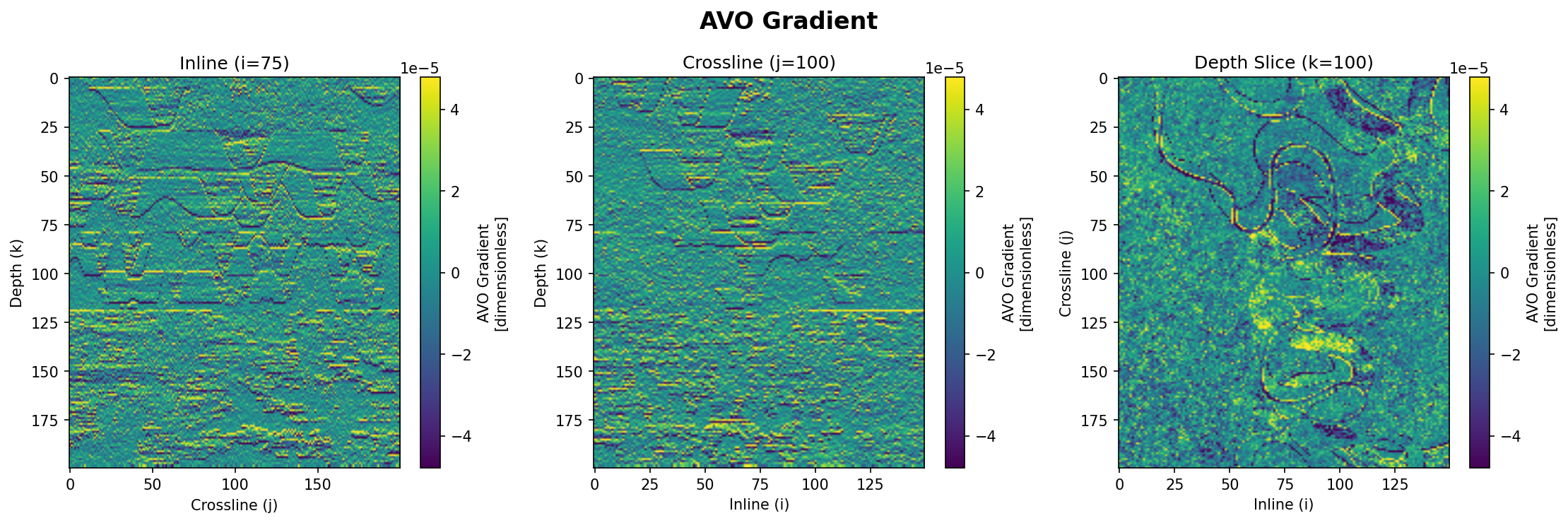
AVO Gradient (B)

The AVO Gradient (B) quantifies how reflection amplitudes change with incidence angle. Because spatial anomalies in B often indicate contrasts in rock elastic properties or fluid substitution, this gradient is central to AVO-based fluid prediction workflows.

Figure 12. AVO Gradient (B). Rate of reflectivity change with incident angle. Captures angle-dependent effects crucial for AVO classification and fluid discrimination.

View 3D Visualization

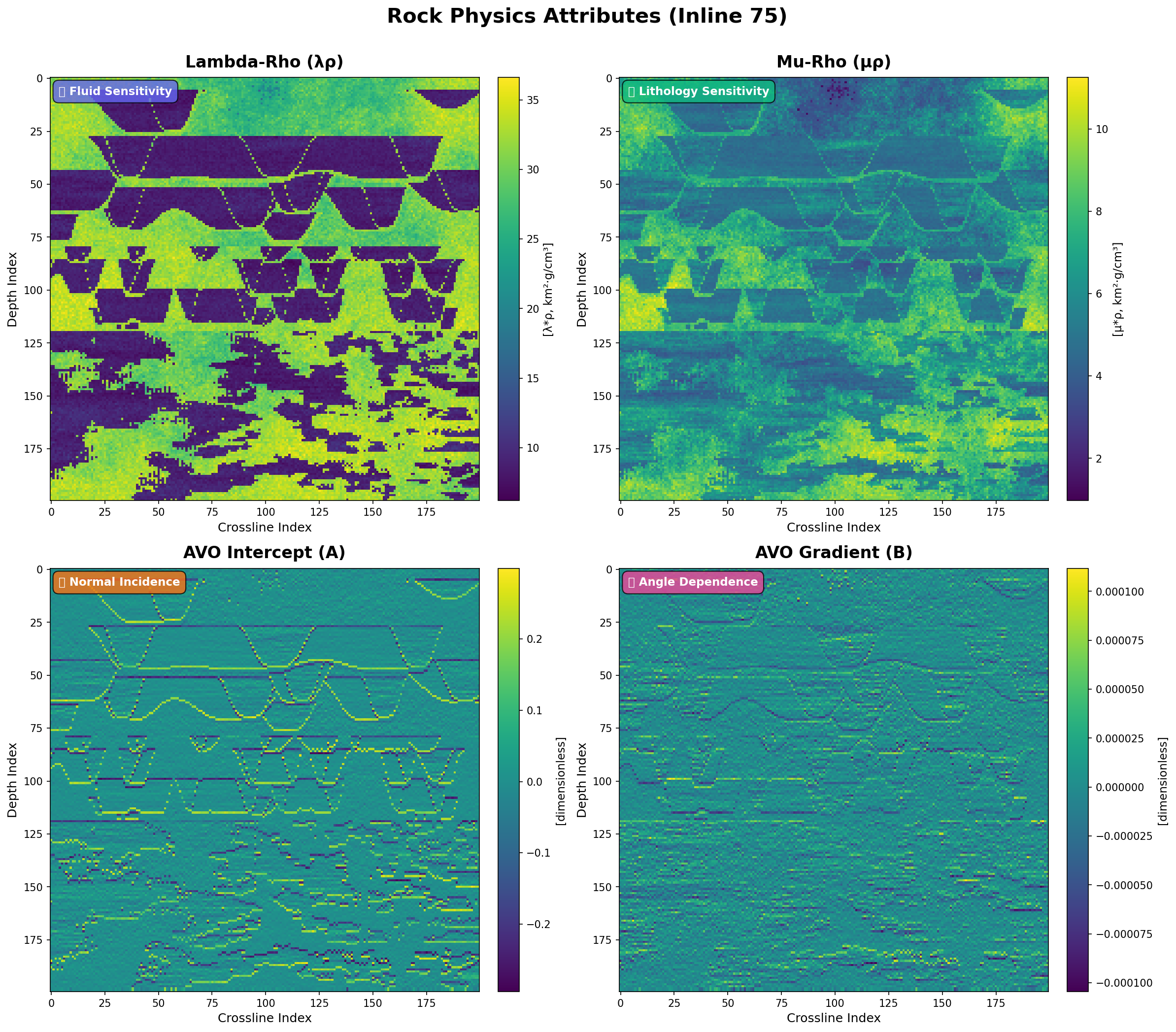
Multi-Attribute Comparison

The figure above presents a 2×2 multi-attribute comparison (Lambda‑Rho, Mu‑Rho, AVO Intercept, and AVO Gradient) at Inline 75. Each panel highlights complementary rock physics responses: λρ emphasises bulk modulus contrasts, μρ isolates rigidity and lithology, while the AVO intercept and gradient capture normal‑incidence and angle‑dependent amplitude behaviour respectively. Use these panels together to cross-validate fluid indicators and facies boundaries across the reservoir section.

Figure 13. Multi-attribute comparison: λρ | μρ on the top row and A | B on the bottom row — shown at Inline 75.

This comparative view along Inline 75 displays four key rock physics attributes essential for AVO analysis and reservoir characterization. The attributes are presented to contrast fluid indicators with rock frame properties. Lambda-Rho ($\lambda\rho$) highlights fluid sensitivity and bulk modulus variations, while Mu-Rho ($\mu\rho$) reveals rock rigidity, allowing for robust lithology discrimination. These are shown alongside the foundational AVO attributes: the Intercept (A), which quantifies normal-incidence reflectivity, and the Gradient (B), which measures changes in reflectivity with angle. Derived from the Aki-Richards approximation, this combined display offers a complementary and powerful dataset for distinguishing fluid effects from lithological changes.

Comparative view of all four key rock physics attributes at Inline 75.

Lambda-Rho (λρ) Fluid sensitivity and bulk modulus indicator

Mu-Rho (μρ) Lithology discrimination and rigidity

AVO Intercept (A) Normal incidence reflectivity term

AVO Gradient (B) Angle-dependent reflectivity change

These attributes are derived from the Aki-Richards linearized approximation andprovide complementary information for reservoir characterization and AVO analysis.

Implementation & Usage

This rock-physics pipeline provides a reproducible method for transforming elastic inputs (Vp, Vs, $\rho$) into advanced attribute volumes. It systematically applies well-documented transforms (like mineral averaging, Constant-Cement, and VRH mixing) and fluid-substitution models (Gassmann, Wood) to generate $\lambda\rho$, $\mu\rho$, AI, SI, Vp/Vs, and AVO attributes in both depth and time domains.

Users manage key parameters, such as sampling, wavelet, and angle ranges, through a central configuration file. To ensure reproducibility, this configuration must be pinned and archived with the final analysis-ready outputs. These outputs include attribute volumes, metadata, and optional 2D/3D visualizations designed for quality control, interpretation, and subsequent AVO or machine-learning workflows.

Running the Code

To execute the analysis, run the provided Python commands from the terminal. You can compute the rock physics attributes in the depth domain by running python -m src --run-tool rock_physics_attributes. To generate the corresponding visualizations, use the command python -m src --run-tool plot_rock_physics_attributes. Alternatively, you can run the complete pipeline, which includes both computation and visualization, with the single command python -m src --run-tool analysis_rock_physics.

# Compute rock physics attributes (depth domain)
python -m src --run-tool rock_physics_attributes

# Generate rock physics plots
python -m src --run-tool plot_rock_physics_attributes

# Complete analysis pipeline (compute + visualize)
python -m src --run-tool analysis_rock_physics